Computer vision has so many applications that is impossible not to be charmed by it. I decided to explore a tiny part of the image analysis world using a fruit as subject.
In the notebook below (which .ipynb file is in my github repository) I use the image segmentation and the edge detector technique to locate any defects on the surface of some apples.
The procedure explained below can be easily applied to other subjects.
- Load Images
- Fruit Segmentation
2.1 Otsu’s Method
2.2 Flood-fill Approach
2.3 Segmented Images - Defects Detection
3.1 Canny Edge Detector
3.2 Erosion - Conclusion
1. Load Images
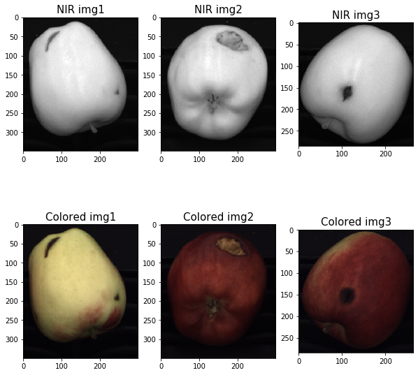
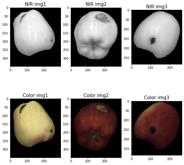
We have three pairs of images acquired through a NIR (Near Infra-Red) and a color camera with a little parallax effect.
We load and display the images below.
import cv2
import numpy as np
from matplotlib import pyplot as plt
%matplotlib inline


#NIR images
img1 = cv2.imread("images/C0_000001.png", cv2.IMREAD_GRAYSCALE)
img2 = cv2.imread("images/C0_000002.png", cv2.IMREAD_GRAYSCALE)
img3 = cv2.imread("images/C0_000003.png", cv2.IMREAD_GRAYSCALE)


#Colored images
img1_c = cv2.cvtColor(cv2.imread("images/C1_000001.png", cv2.IMREAD_COLOR),cv2.COLOR_BGR2RGB)
img2_c = cv2.cvtColor(cv2.imread("images/C1_000002.png", cv2.IMREAD_COLOR),cv2.COLOR_BGR2RGB)
img3_c = cv2.cvtColor(cv2.imread("images/C1_000003.png", cv2.IMREAD_COLOR),cv2.COLOR_BGR2RGB)

#Plot images
plt.figure(figsize=(10,10))
plt.subplot(2,3,1)
plt.imshow(img1, cmap='gray', vmin=0, vmax=255)
plt.title("NIR img1", fontsize = 15)
plt.subplot(2,3,2)
plt.imshow(img2, cmap='gray', vmin=0, vmax=255)
plt.title("NIR img2", fontsize = 15)
plt.subplot(2,3,3)
plt.imshow(img3, cmap='gray', vmin=0, vmax=255)
plt.title("NIR img3", fontsize = 15)
plt.subplot(2,3,4)
plt.imshow(img1_c)
plt.title("Colored img1", fontsize = 15)
plt.subplot(2,3,5)
plt.imshow(img2_c)
plt.title("Colored img2", fontsize = 15)
plt.subplot(2,3,6)
plt.imshow(img3_c)
plt.title("Colored img3", fontsize = 15)
plt.show()
2. Fruit Segmentation
We want to inspect the fruit to locate any defects, thus we need to remove the background and focus the analysis on the fruit (hereinafter called foreground).
One of the most used tool to isolate the foreground is the so called Binary Mask: a binary image having the same size as the target image and defining a region of interest (ROI).
In particular:
- mask pixel values of
1indicate the image pixel belongs to the ROI; - mask pixel values of
0indicate the image pixel is part of the background.
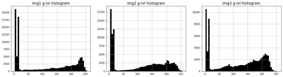
We create our binary masks by thresholding the gray-level histogram of each NIR image displayed below.
#Gray-level histograms
plt.figure(figsize = (20, 5), num = 'Gray-level histograms')
plt.subplot(1,3,1)
plt.hist(img1.flatten(), bins = 50, color = 'black');
plt.ticklabel_format()
plt.grid()
plt.title("img1 g-lvl histogram", fontsize = 15)
plt.subplot(1,3,2)
plt.hist(img2.flatten(), bins = 50, color = 'black');
plt.grid()
plt.title("img2 g-lvl histogram", fontsize = 15)
plt.subplot(1,3,3)
plt.hist(img3.flatten(), bins = 50, color = 'black');
plt.grid()
plt.title("img3 g-lvl histogram", fontsize = 15)
plt.show()
2.1 Otsu’s Method
The three histograms clearly show the background peaks, but the gray-level values are spread over the whole range; thus it’s hard to manually find a correct threshold for each image.
How could we select a meaningful threshold?
One of the most well known approach is the Otsu’s method, which consists in maximizing the between-group variance of the background and the foreground.
Therefore, this method provides the thresholding value which makes both the background and the foreground the most homogeneous as possible.
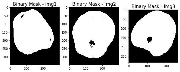
Once we have found the best threshold according to Otsu’s method, we create our binary mask by setting at 0 each pixel classified as background and at 1 each foreground pixel.
The resulting masks exhibit some holes which coincide to the darkest regions of the fruit that have been wrongly classified as background.
It’s not surprising that the thresholding operation misclassified some pixels: as we highlighted, the intensity distribution is quite stretched and therefore the presence of false negatives and false positives is very likely.
# Thresholding with Otsu's method
thresh = 25
maxValue = 1

th1, dst1 = cv2.threshold(img1, thresh, maxValue, cv2.THRESH_OTSU)
th2, dst2 = cv2.threshold(img2, thresh, maxValue, cv2.THRESH_OTSU)
th3, dst3 = cv2.threshold(img3, thresh, maxValue, cv2.THRESH_OTSU);
print("The resulting thresholding values are:\n\n {:0.0f} for img1,\n {:0.0f} for img2,\n {:0.0f} for img3."\
      .format(th1, th2, th3))
The resulting thresholding values are:

 109 for img1,
 98 for img2,
 104 for img3.
#Plot Binary Masks
plt.figure(figsize=(10,10))
plt.subplot(1,3,1)
plt.imshow(dst1 * 255, cmap='gray', vmin=0, vmax=255)
plt.title("Binary Mask - img1", fontsize = 15)
plt.subplot(1,3,2)
plt.imshow(dst2 * 255, cmap='gray', vmin=0, vmax=255)
plt.title("Binary Mask - img2", fontsize = 15)
plt.subplot(1,3,3)
plt.imshow(dst3 * 255, cmap='gray', vmin=0, vmax=255)
plt.title("Binary Mask - img3", fontsize = 15)
plt.show()
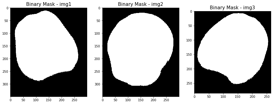
2.2 Flood-fill approach
To correct the false negatives introduced by the thresholding, we use the flood-fill algorithm to fill the connected components in the target image with a specified value.
In the lines below, we use the floodFill function of OpenCV to fill the holes inside our binary masks:
- we set at
1the filling value and we prepare a (h+2) by (w+2) empty mask, where h and w are the dimensions of the original image; - we fill the connected components in the original image and we invert the resulting binary image;
- we combine the original image with the new one to get a Binary Mask without holes.
#Flood fill apporach

#Copy the masks
dst1_floodfill = dst1.copy()
dst2_floodfill = dst2.copy()
dst3_floodfill = dst3.copy()

# Masks used to flood filling
h, w = dst1.shape[:2]
m1 = np.zeros((h+2, w+2), np.uint8)
h, w = dst2.shape[:2]
m2 = np.zeros((h+2, w+2), np.uint8)
h, w = dst3.shape[:2]
m3 = np.zeros((h+2, w+2), np.uint8)

# Floodfill starting from point (0,0) with new value 1
seed_point = (0,0)
newValue = 1

cv2.floodFill(dst1_floodfill, m1, seed_point, newValue);
cv2.floodFill(dst2_floodfill, m2, seed_point, newValue);
cv2.floodFill(dst3_floodfill, m3, seed_point, newValue);

#Invert the resulting images
holes1 = np.invert(dst1_floodfill > 0)
holes2 = np.invert(dst2_floodfill > 0)
holes3 = np.invert(dst3_floodfill > 0)

#Combine the two images to get the final binary masks
mask1 = dst1 | holes1
mask2 = dst2 | holes2
mask3 = dst3 | holes3
#Plot filled masks
plt.figure(figsize=(10,10))
plt.subplot(1,3,1)
plt.title("Binary Mask - img1", fontsize = 15)
plt.imshow(mask1 * 255, cmap='gray', vmin=0, vmax=255)
plt.subplot(1,3,2)
plt.title("Binary Mask - img2", fontsize = 15)
plt.imshow(mask2 * 255, cmap='gray', vmin=0, vmax=255)
plt.subplot(1,3,3)
plt.title("Binary Mask - img3", fontsize = 15)
plt.imshow(mask3 * 255, cmap='gray', vmin=0, vmax=255)
plt.show()
2.3 Segmented Images
We apply the binary masks on both the NIR and the colored images: the resulting images present a completely homogeneous background and the unmodified fruit.
#Create the masks for the colored images
mask1_RGB = cv2.cvtColor(mask1, cv2.COLOR_GRAY2BGR)
mask2_RGB = cv2.cvtColor(mask2, cv2.COLOR_GRAY2BGR)
mask3_RGB = cv2.cvtColor(mask3, cv2.COLOR_GRAY2BGR)

#Apply the masks
m_img1_c = img1_c * mask1_RGB
m_img2_c = img2_c * mask2_RGB
m_img3_c = img3_c * mask3_RGB

Img1 = img1 * mask1
Img2 = img2 * mask2
Img3 = img3 * mask3
# Plot segmented images
plt.figure(figsize=(10,10))
plt.subplot(2,3,1)
plt.imshow(Img1, cmap='gray', vmin=0, vmax=255)
plt.title("NIR img1", fontsize = 15)
plt.subplot(2,3,2)
plt.imshow(Img2, cmap='gray', vmin=0, vmax=255)
plt.title("NIR img2", fontsize = 15)
plt.subplot(2,3,3)
plt.imshow(Img3, cmap='gray', vmin=0, vmax=255)
plt.title("NIR img3", fontsize = 15)
plt.subplot(2,3,4)
plt.imshow(m_img1_c)
plt.title("Colored img1", fontsize = 15)
plt.subplot(2,3,5)
plt.imshow(m_img2_c)
plt.title("Colored img2", fontsize = 15)
plt.subplot(2,3,6)
plt.imshow(m_img3_c)
plt.title("Colored img3", fontsize = 15)
plt.show()
3. Defects Detection
3.1 Canny Edge Detector
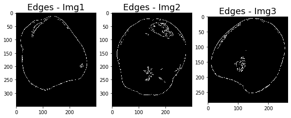
The imperfections show sharp edges and so we can use an edge detector to “draw” their contours.
There exist several edge detectors and all of them are based on finding the discontinuities in brightness. The one we are going to use is named Canny Edge Detector and it is implemented in OpenCV in the Canny function.
Canny function has two parameters (high-threshold and low-threshold) which determine the hysteresis process of thresholding and which have to be carefully tuned.
There are no universal guidelines to select the best parameter values, so we decided to apply the Otsu’s method on the masked NIR image to set the high-threshold parameter and we set the low-threshold equal to half high-threshold.
#Otsu's method
h_th1, _ = cv2.threshold(Img1, thresh, maxValue, cv2.THRESH_OTSU)
h_th2, _ = cv2.threshold(Img2, thresh, maxValue, cv2.THRESH_OTSU)
h_th3, _ = cv2.threshold(Img3, thresh, maxValue, cv2.THRESH_OTSU)

print("The high-threshold values are:\n\n {:0.0f} for Img1,\n {:0.0f} for Img2,\n {:0.0f} for Img3."\
      .format(h_th1, h_th2, h_th3))


#Canny's detector
Canny_1 = cv2.Canny(Img1, h_th1 / 2, h_th1)
Canny_2 = cv2.Canny(Img2, h_th2 / 2, h_th2)
Canny_3 = cv2.Canny(Img3, h_th3 / 2, h_th3)
>>> The high-threshold values are:
>>>
>>> 99 for Img1,
>>> 89 for Img2,
>>> 90 for Img3.
3.2 Erosion
The resulting images show the contours of both the fruit and the imperfections, and we can also notice some spurious edges.
We would like to obtain a binary image with only the fruit defects as foreground, therefore we have to remove the unnecessary parts.
A very useful tool is the erode function of OpenCV, which performs the operation of erosion) on the target image.
# Plot edges found by Canny's detector
plt.figure(figsize=(10,10))
plt.subplot(1,3,1)
plt.imshow(Canny_1, cmap = 'gray')
plt.title("Edges - Img1", fontsize = 15)
plt.subplot(1,3,2)
plt.imshow(Canny_2, cmap = 'gray')
plt.title("Edges - Img2", fontsize = 15)
plt.subplot(1,3,3)
plt.imshow(Canny_3, cmap = 'gray')
plt.title("Edges - Img3", fontsize = 15)
plt.show()
The erode function takes 3 arguments:
- the original image;
- the kernel (the matrix with which image is convolved);
- the number of iterations which will determine the degree of erosion.
For our purpose, we take as kernel a 5 by 5 empty matrix and we set at 5 the number of iterations.
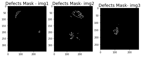
We proceed by eroding the original binary mask (the one generated using Otsu’s thresholding and filled with the flood-fill approach); then we use the eroded binary mask to extract only the imperfections contours from the image provided by the edge detector.
In the lines below we build the ad hoc function defects and we generate the three “defects” images.
#Erosion

def defects(canny_img, mask, kernel_size = (5,5), n_iter = 1):

    #Erosion
    kernel = np.ones(kernel_size, np.uint8)
    eroded_mask = cv2.erode(mask, kernel, iterations = n_iter)

    #Apply mask
    canny_mask = (np.invert(canny_img)*mask).flatten()
    empty = np.zeros(canny_mask.shape)
    i = 0

    for n in eroded_mask.flatten():
        i += 1
        if n :
            if canny_mask[i] == 0:
                empty[i] = 255

    return empty.reshape(canny_img.shape)
defects1 = defects(Canny_1, mask1, n_iter=5)
defects2 = defects(Canny_2, mask2, n_iter=5)
defects3 = defects(Canny_3, mask3, n_iter=5)
# Plot the defects
plt.figure(figsize=(10,10))
plt.subplot(1,3,1)
plt.imshow(defects1, cmap = 'gray')
plt.title("Defects Mask - img1", fontsize = 15)
plt.subplot(1,3,2)
plt.imshow(defects2, cmap = 'gray')
plt.title("Defects Mask- img2", fontsize = 15)
plt.subplot(1,3,3)
plt.imshow(defects3, cmap = 'gray')
plt.title("Defects Mask- img3", fontsize = 15)
plt.show()
4. Conclusion
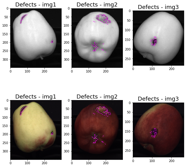
We use the “defects” images to draw the detected defects both on the NIR and the colored images.
As expected, in the resulting colored images the detected defects do not perfectly match the real imperfections contours: this is because we apply the edge detector on the NIR images and, as mentioned at the beginning, the pairs of images are affected by the parallax effect.
We also notice that the apple sepals have been classified as defects in img2: the sepals exhibit a sharp change in intensity wich has been detected by Canny Edge Detector.
def draw_defects_Gray(img, defects):

    img_RGB = cv2.cvtColor(img, cv2.COLOR_GRAY2BGR)
    h,w,bpp = img_RGB.shape

    for py in range(0,h):
        for px in range(0,w):
            if(defects[py][px]):
                img_RGB[py][px][0] = 255
                img_RGB[py][px][1] = 0
                img_RGB[py][px][2] = 255

    return img_RGB

def draw_defects_RGB(img, defects):

    h,w,bpp = img.shape
    img_copy = img.copy()

    for py in range(0,h):
        for px in range(0,w):
            if(defects[py][px]):
                img_copy[py][px][0] = 255
                img_copy[py][px][1] = 0
                img_copy[py][px][2] = 255

    return img_copy
defects_img1 = draw_defects_Gray(img1, defects1)
defects_img2 = draw_defects_Gray(img2, defects2)
defects_img3 = draw_defects_Gray(img3, defects3)

defects_img1_RGB = draw_defects_RGB(img1_c, defects1)
defects_img2_RGB = draw_defects_RGB(img2_c, defects2)
defects_img3_RGB = draw_defects_RGB(img3_c, defects3)
# Plot colored images with defects
plt.figure(figsize=(10,10))
plt.subplot(2,3,1)
plt.imshow(defects_img1)
plt.title("Defects - img1", fontsize = 15)
plt.subplot(2,3,2)
plt.imshow(defects_img2)
plt.title("Defects - img2", fontsize = 15)
plt.subplot(2,3,3)
plt.imshow(defects_img3)
plt.title("Defects - img3", fontsize = 15)
plt.subplot(2,3,4)
plt.imshow(defects_img1_RGB)
plt.title("Defects - img1", fontsize = 15)
plt.subplot(2,3,5)
plt.imshow(defects_img2_RGB)
plt.title("Defects - img2", fontsize = 15)
plt.subplot(2,3,6)
plt.imshow(defects_img3_RGB)
plt.title("Defects - img3", fontsize = 15)
plt.show()
This work is licensed under a Creative Commons Attribution-ShareAlike 3.0 Unported License.