What is the queueing theory?
In a day routine there are lots of situations where we could find ourselves stuck in a queue. Let’s think about the flow of commuters or about a shopping centre: both situations represent potential sources of queues.
There is a mathematical structure focused on the study of queues: the Queueing Theory (QT for brevity) developed in the 20th century [1]. QT is applied in many fields from telecommunication to traffic engineering, from industrial engineering to optimization of public and private services.
The key elements of a queueing model are customers and servers: the former refer to anything that arrives at a facility and require a service (such as people, bits of information, trucks, etc.); the latter refer to any resource that provide the requested service (front office, cpu, runway and so on).
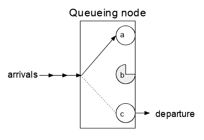
A queue can be schematized with a queueing node, where customers arrive, wait a little in the queue and depart after being processed by one or more servers.
Types of queue
Queueing systems are not all equal: they may differ in the queueing discipline, in the number of servers, in the arrival rate and so on.
In the 50s D. G. Kendall proposed a compact notation to represent the different queueing models which is used nowadays.
Kendall’s notation[1] has 6 parameters divided by a slash:
A/S/c/K/N/D
- A refers to the arrivals distribution in time;
- S refers to the services time distribution;
- c is the number of servers at the node;
- K is the system capacity (maximum length of the queue) ;
- N is the size of the calling population (the population which the customers come from);
- D refers to the queueing discipline.
When the last 3 parameters are not specified, we assume that K = ∞, N = ∞ and D = FIFO (First-In First-Out).
M/M/c and the hospital reception
One of the simplest queue systems is the M/M/c queue, where the arrivals are governed by a Poisson process and the service times have an exponential distribution.
The letter M stands for Markovian or memoryless, which means that the system is a Markov chain: its future state is related only to its present state.
The number of servers at the queue node is a finite number c, so if there are less than c customers, some of the servers will be idle. On the contrary, if there are more than c customers, the customers queue in the infinite buffer ( K = ∞ ).
There are two fundamental parameters describing this system:
- the rate of arrivals λ, which determines the inverse of the mean of the Poisson distribution of arrivals ;
- the service rate µ, which characterizes the exponential distribution mean of service times.
Let’s now imagine an ideal hospital with an infinite number of front offices ready to serve a potentially infinite number of patients.
The patients go to our hospital and ask for different services which require different time to be computed. Each front office is able to provide any required service and we believe in the “FIFO philosophy“: the first patient entering the hospital is the first to be served.
We can model our ideal hospital as a M/M/c queue and we can simulate the system using an agent-based simulation.
NetLogo Simulation
We use NetLogo 6.0.4 to create the agent-based simulation of our hospital reception based on the interaction between two different breeds of agents: patients and front offices.
In each iteration the first patient in the queue reaches an available (green) front office to request for a service; the front offices turns red and remains busy until the requested service is provided. Then, the served patient leaves the reception and the front office turns available again.
In the simulation you can set the number of front offices, the arrival rate λ and the service rate µ to observe the system behaviour with different configurations.
You can run the model on your browser:
- click here to run the simulation;
- in the section Model Info you can find the useful HOW TO USE IT section and some other information;
- by clicking on the Mode button at the top-left corner you can switch to the Authoring mode and manipulate the model;
- if you would like to download the .nlogo file, simply use the Export button at the top-right corner.
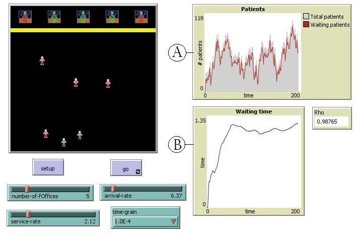
Simulation overview
The reception is displayed on the left, while on the right you can find:
- the chart A showing the total number of patients and the number of waiting patients;
- the chart B showing the average time spent in queue;
- the value Rho, which is strictly related to the equilibrium condition of our system.
This project is part of one of my Master’s degree exams at the Università degli Studi di Torino (see professor Terna’s website to know more).
Here you can find my more detailed review of the project.
Bibliography
[1] (2016) J. Sztrik, Basic Queueing Theory , University of Debrecen, Faculty of Informatics
[2] (2013) Kendall’s Notation. In: Gass S.I., Fu M.C. (eds) Encyclopedia of Operations Research and Management Science. Springer, Boston, MA