One of the most well known graphical modeling classes for reasoning with uncertainty is the so called Bayesian network, which relies on the Bayesian inference to answer to probabilistic queries. In a Bayesian network the variables and the conditional dependencies among them are represented by a directed acyclic graph (DAG).
Let’s define a toy Bayesian network exploring some features of the pgmpy library.
- Introduction
- Define the model
- Conditional Probability Distributions
- Independence
- Markov Blanket
- d-separation principle
- Inference
- Exact inference
- Approximate inference
Introduction
Let’s consider a publishing house which has to commission a translation, how should it select a valid translator?
In a simplified world the publishing house would take into account the academic results, and the speaking and writing skills of a candidate. So let’s suppose that the candidates are evaluated according to:
- their degree in the target language (with or without honors);
- their fluency in the target language (being bilingual or not);
- their writing skills.
The above concepts can be easily encoded with Boolean variables:
- Grad_with_honors(Yes/No)
- Bilingual (Yes/No)
- Writing (Poor/High writing skills)
Let’s also suppose that the writing skills and the graduation are affected by the number of books read by the candidate:
- Reading (less/more than 3 books per month)
Define the model
The first step consists in building the structure of our model, that is to define the relations between the involved variables.
In the following lines we define the network model using pgmpy library and we display the resulting graph using networkx.
from pgmpy.models import BayesianModel

model = BayesianModel([('Grad_with_honors', 'Commission'),
                       ('Bilingual', 'Commission'),
                       ('Writing', 'Commission'),
                       ('Bilingual', 'Grad_with_honors'),
                       ('Reading', 'Grad_with_honors'),
                       ('Reading', 'Writing')
                       ])

#Network nodes and out-edges
nodes = list(model.nodes())
edges = list(model.edges())
import matplotlib.pyplot as plt
import networkx as nx
import numpy as np
np.random.seed(8)
DAG = nx.DiGraph()
DAG.add_edges_from(edges)
fig = plt.figure(figsize = (10,10))
pos = nx.spring_layout(DAG) #Position nodes computed by using Fruchterman-Reingold force-directed algorithm.
nx.draw_networkx_nodes(DAG, pos=pos, node_color='turquoise')
nx.draw_networkx_labels(DAG, pos=pos)
nx.draw_networkx_edges(DAG, pos=pos, edge_color='black', width = 1.5, arrows=True)
plt.show()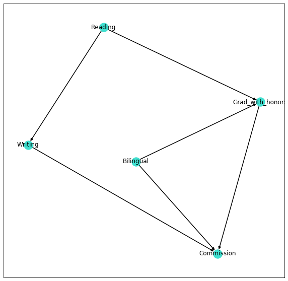
Conditional Probability Distributions
In order to make predictions with our model, we need to define the conditional probability distribution (CPD) of each variable.
By looking at the network shown above, we can easily conclude that:
- Reading and Bilingual have only prior probabilities ⟹ 2 entrances in the corresponding CPD tables;
- Writing, Grad_with_honors and Commission have conditional probabilities ⟹ 4,8 and 16 entrances in the corresponding CPD tables.
from pgmpy.factors.discrete import TabularCPD

#Less/more than 3 books per month
reading_cpd=TabularCPD('Reading',2,[[.7,.3]])

#Not bilingual/bilingual
bilingual_cpd=TabularCPD('Bilingual',2,[[.85,.15]])

#Poor/High writing skills given Reading
writing_cpd=TabularCPD('Writing',2,[[.85,.4],[.15,.6]],
                       evidence=['Reading'],
                       evidence_card=[2])

#Graduation withot/with honors given Reading and Bilingual
graduation_cpd=TabularCPD('Grad_with_honors',2,[[.65,.3,.55,.2],[.35,.7,.45,.8]],
                       evidence=['Bilingual','Reading'],
                       evidence_card=[2,2])

#Not getting/getting the commission given Writing, Bilingual and Grad_with_honors
commission_cpd=TabularCPD('Commission',2,[[.95,.73,.7,.23,.35,.20,.28,.1],[.05,.27,.3,.77,.65,.8,.72,.9]],
                       evidence=['Grad_with_honors','Bilingual','Writing'],
                       evidence_card=[2,2,2])

model.add_cpds(reading_cpd,
               bilingual_cpd,
               writing_cpd,
               graduation_cpd,
               commission_cpd)

#Verify the model correctness by:
#  -checking if the sum of the probabilities for each state is equal to 1;
#  -checking if the CPDs associated with nodes are consistent with their parents.
if model.check_model():
    print("No errors in the defined model.")
>>> No errors in the defined model.Independence
To reason about independence relations among the nodes of a Bayesian network we can rely on the Markov blanket and the d-separation principle.
Markov blanket
The Markov blanket of a given node consists in the set of its parents, its children and its children’s other parents. Moreover, given the Markov blanket of a node, the node itself becomes independent from any other nodes of the network.
For brevity, we display only the Reading node (turquoise) with its Markov blanket (yellow) and the remaining node (gray).
leaves = model.get_leaves()
markov_blanket = {}

for node in nodes:
    if not node in leaves:
        markov_blanket[node] = model.get_markov_blanket(node)
        print("-"*80,"\n")
        print(node, "\nMarkov blanket ->", markov_blanket[node])

        nx.draw_networkx_nodes(DAG, pos, nodelist=[node], node_color='turquoise')
        nx.draw_networkx_nodes(DAG, pos, nodelist=markov_blanket[node], node_color='yellow')
        nx.draw_networkx_nodes(DAG, pos,
               nodelist = [n for n in nodes if n not in markov_blanket[node] and n != node],
               node_color='grey')
        nx.draw_networkx_labels(DAG, pos)
        nx.draw_networkx_labels(DAG, pos)
        nx.draw_networkx_edges(DAG, pos, edge_color='black', width = 2.0, arrows=True)
plt.show()d-separation principle
The d-separation principle allows us to determine whether a set X of variables is independent of another set Y, given a third set Z.
The main idea is to associate dependence with connectedness, and independence with separation. Therefore, the d-separation is strictly related to the concept of active-trail in a directed graph:
if there is no active trail between two variables X and Y, then X and Y are d-separated.
As an example, let’s consider the V-structure made up of the variables Bilingual and Reading and let’s verify its correctness using the method is_active_trail.
print(model.is_active_trail('Bilingual','Reading'))
print(model.is_active_trail('Bilingual','Reading','Grad_with_honors'))
print(model.is_active_trail('Bilingual','Reading','Commission'))

>>> False
>>> True
>>> True
Let’s now determine the marginal and conditional independence relations in our network by using the get_independecies method, which is based on the d-separation principle.
model.get_independencies()
>>>
   (Grad_with_honors _|_ Writing | Reading)
   (Grad_with_honors _|_ Writing | Reading, Bilingual)
   (Commission _|_ Reading | Grad_with_honors, Writing, Bilingual)
   (Bilingual _|_ Writing, Reading)
   (Bilingual _|_ Reading | Writing)
   (Bilingual _|_ Writing | Reading)
   (Bilingual _|_ Writing | Grad_with_honors, Reading)
   (Writing _|_ Bilingual)
   (Writing _|_ Grad_with_honors, Bilingual | Reading)
   (Writing _|_ Bilingual | Grad_with_honors, Reading)
   (Writing _|_ Grad_with_honors | Reading, Bilingual)
   (Reading _|_ Bilingual)
   (Reading _|_ Bilingual | Writing)
   (Reading _|_ Commission | Grad_with_honors, Writing, Bilingual)
Inference
There are two classes of inference methods: the exact inference and the approximate inference. In the former, we analytically compute the conditional probability distribution over the variables of interest using the posterior probability distributions. In the latter, we approximate the required posterior probability distributions using sampling methods or optimization techniques.
Thanks to the inference methods, we can execute:
- a conditional probability query (i.e. asking for the probability that a node X has a particular value x given the evidence of Y being equal to y, formally P(X=x∣Y=y));
- a MAP query (i.e. asking for the most likely explanation for some evidence – Maximum A-posteriori Probability).
Exact inference
A very well known algorithm to perform exact inference on graphical models is the Variable Elimination (VE).
In the lines below we test VE by asking for:
- the prior probability distribution of Commission
- the probability distribution of Commission given the evidence Writing = 0;
- the probability distribution of Writing and Bilingual given Commission = 0;
- the MAP of the evidence Reading=>3.
from pgmpy.inference import VariableElimination

exact_inference = VariableElimination(model)

query1 = exact_inference.query(['Commission'])
query2 = exact_inference.query(['Commission'],{'Writing':0})
query3 = exact_inference.query(['Writing', 'Bilingual'], {'Commission':0})
query4 = exact_inference.map_query(['Commission', 'Writing', 'Grad_with_honors'], {'Reading':1})

print('\nP(Commission)\n\n',query1)
print('\n\nP(Commission|Writing=poor)\n\n',query2)
print('\n\nP(Reading, Bilingual|Commission=no)\n\n',query3)
print('\n\nMAP of Reading = > 3\n\n',query4)
>>> P(Commission)
+---------------+-------------------+
| Commission | phi(Commission) |
+===============+===================+
| Commission(0) | 0.5901 |
+---------------+-------------------+
| Commission(1) | 0.4099 |
+---------------+-------------------+
>>> P(Commission|Writing=poor)
+---------------+-------------------+
| Commission | phi(Commission) |
+===============+===================+
| Commission(0) | 0.6720 |
+---------------+-------------------+
| Commission(1) | 0.3280 |
+---------------+-------------------+
>>> P(Reading, Bilingual|Commission=no)
+------------+--------------+--------------------------+
| Writing | Bilingual | phi(Writing,Bilingual) |
+============+==============+==========================+
| Writing(0) | Bilingual(0) | 0.7258 |
+------------+--------------+--------------------------+
| Writing(0) | Bilingual(1) | 0.0884 |
+------------+--------------+--------------------------+
| Writing(1) | Bilingual(0) | 0.1754 |
+------------+--------------+--------------------------+
| Writing(1) | Bilingual(1) | 0.0103 |
+------------+--------------+--------------------------+
>>> MAP of Reading = > 3
{'Commission': 1, 'Writing': 1, 'Grad_with_honors': 1}
3.2 Approximate inference
The main problem in performing exact inference is that it’s carried out with posterior probabilities which are not always tractable. The approximate inference addresses this issue by sampling form the untractable posterior (stochastic methods) or by approximating the posterior with a tractable distribution (deterministic methods).
In the lines below we compare three sampling methods (Weighted Likelihood (WL), Rejection Sampling (RS) and Gibbs Sampling (GS)) using the VE result as reference. We query the model for P(Reading >= 3| Bilingual=Yes,Commission = No) and we run 10 experiments with an increasing number of samples.
# Exact Inference

query = exact_inference.query(['Reading'], {'Bilingual' : 1,'Commission' : 0})
print("\nP(Reading | Bilingual = yes, Commission = no)\n\n",query)

reference_prob = query.values[1]
>>> P(Reading | Bilingual = yes, Commission = no) +------------+----------------+ | Reading | phi(Reading) | +============+================+ | Reading(0) | 0.8292 | +------------+----------------+ | Reading(1) | 0.1708 | +------------+----------------+
from pgmpy.sampling import BayesianModelSampling
from pgmpy.factors.discrete import State
from pgmpy.sampling import GibbsSampling

BMS_inference = BayesianModelSampling(model)
gibbs = GibbsSampling(model)

def prob_WL(samples,variable):
    return round(np.sum(np.dot(samples[variable],samples['_weight']))/np.sum(samples['_weight']),2)

def prob_Gibbs(samples):
    return (samples.query('Reading == 1 & Bilingual == 1 & Commission == 0').shape[0]
                /
            samples.query('Bilingual == 1 & Commission == 0').shape[0])

def run_experiment(sample_size):
    # Sample
    samples_WL = BMS_inference.likelihood_weighted_sample(
                      evidence = evidence,
                      size=sample_size,
                      return_type='recarray')
    samples_RS = BMS_inference.rejection_sample(
                      evidence = evidence,
                      size=sample_size,
                      return_type='recarray')
    samples_GS= gibbs.sample(size = size)

    # Probability
    results_WL = prob_WL(samples_WL,'Reading')
    results_RS = np.recarray.mean(samples_RS['Reading'], axis=0)
    results_GS = prob_Gibbs(samples_GS)

    # Return results
    return np.array([(sample_size,
                      results_WL,
                      results_RS,
                      results_GS)],
                    dtype=[('sample_size', '<i8'),
                           ('results_WL', '<f8'),
                           ('results_RS', '<f8'),
                           ('results_GS', '<f8')])
# Approximate Inference

approximate_results = np.array([], dtype=[('sample_size', '<i8'),
                           ('results_WL', '<f8'),
                           ('results_RS', '<f8'),
                           ('results_GS', '<f8')])
initial_size = 2
final_size = 5
num = 10
evidence = [State('Bilingual',1), State('Commission',0)]

# Run the experiment
for size in np.logspace(initial_size, final_size, num=num, dtype='<i8'):
    approximate_results=np.append(approximate_results,run_experiment(size))

print(approximate_results)
>>>
[(   100, 0.19, 0.19      , 0.5       )
 (   215, 0.18, 0.20465116, 0.2       )
 (   464, 0.17, 0.17672414, 0.15384615)
 (  1000, 0.17, 0.18      , 0.27777778)
 (  2154, 0.16, 0.18709378, 0.23931624)
 (  4641, 0.17, 0.16418875, 0.18181818)
 ( 10000, 0.17, 0.1633    , 0.18197574)
 ( 21544, 0.17, 0.16928147, 0.17205998)
 ( 46415, 0.17, 0.17483572, 0.17439632)
 (100000, 0.17, 0.17133   , 0.17571552)]
As shown in the figure below, the probability inferred using the stochastic methods progressively converges to the reference value.
# Compare the results

plt.figure(figsize=(10,10))
plt.grid(True)
plt.title('\nP(Reading = > 3 | Bilingual = yes, Commission = no)\n')
plt.xlabel("# samples (log scale)")

sizes = approximate_results['sample_size']
results_WL = approximate_results['results_WL']
results_RS = approximate_results['results_RS']
results_GS = approximate_results['results_GS']

plot_WL, = plt.semilogx(sizes, results_WL, 'yo--', label="WL")
plot_RS, = plt.semilogx(sizes, results_RS, 'bo--', label="RS")
plot_GS,= plt.semilogx(sizes, results_GS, 'go--', label="GS")
plot_VE,= plt.semilogx(sizes, reference_prob*np.ones(len(sizes)),'r', label="VE - reference value")

plt.legend(handles=[plot_WL, plot_RS, plot_GS, plot_VE])
plt.show()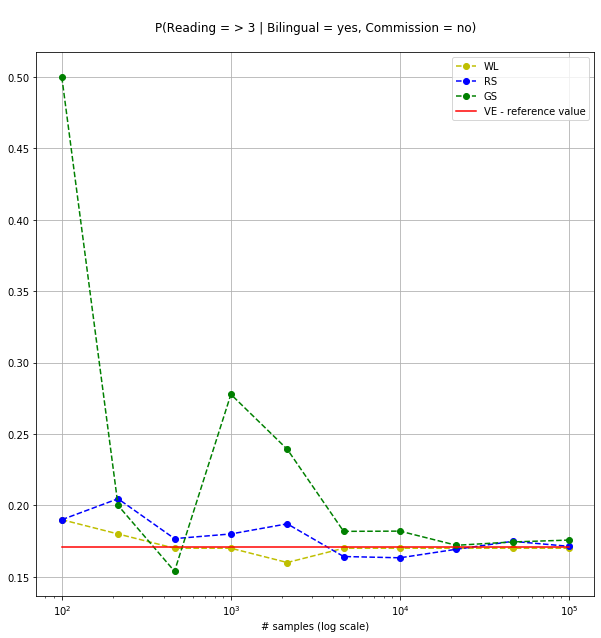
This project was part of my Fundamentals of AI and Knowledge Representation exam of the Master’s degree in Artificial Intelligence, University of Bologna.
This work is licensed under a Creative Commons Attribution-ShareAlike 3.0 Unported License.