Natural Language Processing (NLP) is a multidisciplinary research area which focuses on understanding, analyzing and generating human languages. Since natural languages are complex phenomena, NLP is a very rich field that try to solve many different tasks: from Speech Recognition to Sentiment Analysis, from Text Summarization to Machine Translation.
As part of Data Mining, Text Mining and Big Data Analytics exam, I performed a sentiment analysis on a large supervised dataset of tweets (Sentiment140 dataset).
Here you can find the notebook of this project, which is focused on exploring 3 different text representations (Bag-of-Words, TF-IDF and Word2Vec) and comparing 3 classification models (Multinomial Naive Bayes, Logistic Regression, Multi-layer Perceptron (MLP)).
You can directly run the notebook on Colab here.
In the following sections I briefly described some of the NLP techniques that I used
If you are interested, you can find a more extensive description, as well as the training configuration and the results, in this notebook.
- Word Cloud
- Tweets Features Extraction
- Text Preprocessing
- Text Representations
- Bag-of-Words
- TF-IDF
- Word2Vec
Word Cloud
To have a first look at our data, we can rely on a very common visual representation named Word Cloud.
In a word cloud, each word is written with a font size proportional to its frequency in the text ( i.e. bigger term means higher frequency). Thus, Word Cloud is very useful to quick perceive the most prominent terms in a text.
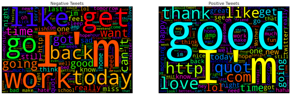
In Figure 1, you can see the word cloud of negative tweets (on the left) and positive tweets (on the right).
By looking at these two images, we can make some considerations:
- in positive word cloud there are terms like good, love, thank, and also lol, great, happy, fun; while in negative word cloud we read words like work, back, bad, and also miss, hate, sorry, sad, tired. Thus, even with this preliminary inspection, we are able to observe some difference between the corpus of positive and negative tweets.
- As expected, some very frequent terms such as day, now, going are in common to the word clouds, since they can be used in both the contexts.
By removing nltk list of stopwords (plus term day), some interesting features springing up in the two word clouds (Figure 2):
- I’m is by far one of the most frequent tokens in both the word clouds; this may underline the self-centered nature of tweets content. Moreover, the token good is much more important in positive tweets than in negative ones.
- The relevance of http and com tokens in positive word cloud may suggest that positive tweets have a higher number of external links with respect to negative ones: this could be an interesting feature to explore more (see next section).
Tweet Features Extraction
Tweets are not only made of plain words, but they may contain links, mentions, emoji, etc. All these elements can be extracted and used as additional features for an NLP task.
Let’s define a list of potential features we want to extract from each tweet:
- number of words (
n_words) - number of uppercase words (
n_capitals) - number of question or exclamation marks (
n_qe_marks) - number of hashtags (
n_hashtags) - number of mentions to other Twitter accounts (
n_mentions) - number of links (
n_urls) - number of emoji (
n_emoji)
To extract these features from the text, we define ad-hoc regular expressions:
- number of words
\w+(match any word) - number of uppercase words
\b[A-Z]{2,}\b(match any uppercase word of 2 or more letters) - number of question or exclamation marks
!|\?(match any question/exclamation mark) - number of hashtags
#\w+(match any word preceded by “#“) - number of mentions
@\w+(match any word preceded by “@”) - number of links
http.?:\/\/[^\s]+[\s]?(match any sequence of characters starting with “http” and containing “:\\“) - number of emoji
_+[a-z_&]+_+(match any sequence made of lowercase letters or “&” and “_“delimited by “__“
Once we have extracted the features, we can perform a two sample Z-test on each of them to verify whether the difference between the mean of the two populations (POSITIVE and NEGATIVE tweets) is statistically significant: if a feature passes the test, than we keep it as a new feature for our classification task, otherwise we discard it.
NOTE
Regarding n_emoji, before counting the regex matches, we pick each emoji and transform it into the corresponding string using the demojize function of module emoji with delimiters parameter set to (__,__). Thus, for example:
"👍""__thumbs_up__""😯""__hushed_face__"
Text Preprocessing
The corpus we are going to work with is a perfect example of unstructured text data that needs to be preprocessed in order to be properly used in a NLP task.
Let’s define and apply a sequence of operations to preprocess each tweet:
- Mentions Removal
- URLS Removal
- Digits Removal
- Lowercase
- Expand Contractions
- Punctuation Removal
- Emoji Transformation
- Stopwords removal or Short terms filtering
- Stemming
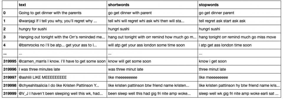
In Table 1 you can find a sample of original tweets and preprocessed ones.
Some of the above mentioned steps are straightforward, but others deserve a closer look:
5. Expand Contractions
We rely on contractions library to expand English contractions such as ‘you’re’ ‘you are’, ‘they won’t’
‘they will not’, and so on.
7. Emoji Transformation
As already described in Tweet Features Extraction, we pick each emoji and transform it in the corresponding string using the demojize function of module emoji. For example:
"👍""::thumbs_up::""😯""::hushed_face::"
Then, we remove : and keep _ in order to have one single word for each emoji.
8. Stopwords removal or Short terms filtering
We test two different pre-processing strategies:
- Remove English stopwords: we use
ntlklist of English stopwords to prune out words which are usually not really informative (articles, auxiliary verbs, conjunctions, etc.). The effectiveness and correctness of this widely used strategy strictly depend on the dataset characteristics. - Filter out very short terms: we discovered that our corpus is plenty of short and meaningless terms composed by 1 or 2 letters. Thus, instead of removing stopwords, we filter out terms shorter than 3 letters or contained in a customized list of very frequent and not highly meaningful terms. By doing so we are able to filter out typos, articles and prepositions without loosing terms which may be meaningful in our application.
NOTE
The customized list of terms used in Filter out very short terms have been defined by looking at the most frequent terms which are present in both positive and negative word clouds.
9. Stemming
Stemming maps different forms of the same word to a common “stem” – for example, the English stemmer maps connection, connections, connective, connected, and connecting to connect. [source]
As stemmer we use Snowball, a class of stemmer algorithms developed by Martin Porter (more info here). We rely on nltk.stem.snowball implementation to efficiently use this algorithms in our process.
Text Representation
We cannot directly feed the unstructured text data into our classifiers, we first need to transform them into numerical objects. But how? There exist several methods to represent the a corpus of documents numerically, and in this project we explore and compare three of them: Bag-of-Words, TF-IDF and Word2Vec.
Bag-of-Words
BoW model is one of the simplest text representation technique: each document is represented as a N-dimensional vector, where N is the total number of tokens in the whole corpus (a token may be a single word/character or a n-gram, with n > 2 ). Each vector component corresponds to the occurrence of the corresponding token into the current document; thus, we end up with a token-document matrix of counts.
The main drawbacks of BoW are that 1) it produces a sparse representation, since many words may not appear in a given document (frequency = 0); 2) it cannot capture phrases and multi-word expressions, effectively ignoring any word order dependence; 3) it may give to much importance to common terms, which appear many times in the corpus, ignoring rarer terms.
TF-IDF
TF_IDF model relies on both term frequency (TF) and inverse document frequency (IDF) in order to make term relevance increasing with the number of occurrences in the given document (TF) and decreasing with the number of occurrences in all the documents in the corpus (IDF):

Each document d is encoded with a N-dimensional vector which components are the tf-idf values of the corresponding tokens (i.e. di = tfidf(ti, d, D) where ti is the i-th token in the vocabulary of corpus D).
Thanks to TF-IDF, we are able to prevent rarer words to be shadowed by very frequent and not so meaningful terms.
Word2Vec
Word2Vec is a word embedding model that learns semantic associations among words from a large corpus of text. It takes a text corpus as input and produces the word embedding vectors as output.
As first, the algorithm constructs the vocabulary of the corpus, then the neural network learns a vector representation for each word.
To better understand this model, let’s consider the example illustrated in Figure 3 (source) with a vocabulary of 10K words:
- the input word “ants” is encoded as a one-hot vector of
components with a
in the position corresponding to the input word itself, and
in all of the other positions;
- the output of the network is a single vector
with
is the probability that a randomly selected word nearby “ants” correspond to the word in position
in the vocabulary.
Figure 3: McCormick, C. (2016, April 19). Word2Vec Tutorial – The Skip-Gram Model. Retrieved from http://www.mccormickml.com
CBOW and Skip-gram
Word2Vec is based on two main learning algorithms: continuous bag-of-words (CBOW) and skip-gram, which can be considered as mirrored versions of each other (Figure 4).
- CBOW tries to predict a single word from a fixed window size of context words;
- Skip-gram does the opposite: it tries to predict several context words from a single input word.
CBOW is faster than Skip-gram, but Skip-gram is better in capturing better semantic relationships, while CBOW learns better syntactic associations.
Moreover, since Skip-gram relies on single words input, it is less prone to overfit frequent words. In fact, even if frequent words are presented more times than rare words during the training, they still appear individually in Skip-gram. On the contrary, CBOW is more prone to overfit frequent words, since they appear several time along with the same context.
Negative Sampling
In the notebook, we rely on negative sampling to speed up the training. Let’s describe in brief the reason behind Negative Sampling and how it works.
Problem:
Training a neural network means taking a training example and adjusting all of the neuron weights slightly so that it predicts that training sample more accurately. In other words, each training sample will tweak all of the weights in the neural network.
In Word2Vec the last layer is a softmax function, thus, for every training sample, the calculation of the final probabilities using the softmax is quite an expensive operation as it involves a summation of scores over all the words in our vocabulary for normalizing.
Moreover, in Word2Vec training, for each training sample only the weights corresponding to the target word might get a significant update. Conversely, the weights corresponding to non-target words would receive a marginal or no change at all, i.e. in each pass we only make very sparse updates.
Solution:
Negative Sampling tries to address the above-mentioned problem by having each training sample only modify a small percentage of the weights, rather than all of them.
In fact, with negative sampling, we are randomly select just a small number of “negative” words (i.e. words for which we want the network to output a 0 for) to update the weights for. We will also still update the weights for our “positive” words (words in the current window).