Simulated Annealing

The core of many AI algorithms is an optimization problem, that is finding the optimum of a given objective function under some constraints. So, anytime we have to tune some parameters according to a loss or gain function, we are dealing with an optimization problem.

There are many subfields of the mathematical optimization discipline and they differ in terms of objective function, constraints and variables domain:

• Linear Programming
• Non-linear Programming
• Integer Programming
• Stochastic Programming
• …

There is a huge number of optimization algorithms, with different structures and applications, but I’d like to describe you the Simulated Annealing, a metaheuristic algorithm.

A natural inspiration

Many metaheuristic algorithms are inspired by natural processes: the Genetic Algorithm, for example, is inspired by the natural selection process, while the Particle Swarm Optimization by some animal behaviours.

Simulated Annealing (hereinafter SA) is among the first metaheuristic algorithms (Kirkpatrick et al., 1983) and it was essentially an extension of the traditional Metropolis–Hastings algorithm. The basic idea of SA is to use random search in terms of a Markov chain, which not only accepts better solutions, but also keeps some worsening solution according to a designed acceptance probability function [1] .

Kirkpatrick’s group was inspired by the analogy between an optimization problem and the physical annealing process, which consists in slowly cooling down a material to remove its imperfections. This process causes a reduction of the Gibbs free energy and here is the core of the analogy mentioned above: we slowly decrease the SA control parameter (temperature) to reduce the energy, i.e. to minimize the objective function. The temperature parameter is crucial for controlling the degree of intensification and diversification during the search, and so for determining the efficiency of the algorithm [2].

How does SA work?

Let’s introduce a bit of notation to help us understanding the algorithm:

• s is the current solution;
• e(s) is the energy of the solution s;
• T is the current temperature;
• s* is the candidate new solution;
• Δe is the difference in energy of two solutions;
• p(Δe, T ) is the acceptance probability function;

The algorithm proceeds with the following steps:

1. start from an initial random point s = s₀ , with the initial temperature T = T₀ ;
2. generate a candidate new solution s*;
3. compute Δe = e(s*) – e(s);
4. if Δe < 0, then s = s*; otherwise accept or reject s* as the new solution according to p(Δe, T );
5. decrease the temperature;
6. check for reanniling;
7. repeat from step 2 to step 6 until a stopping condition is satisfied.

There exist many different possible implementations of the SA algorithm, since each step mentioned above can be customized. We can set the initial temperature and design how our algorithm will generate the new solution. We can design the acceptance probability function and the cooling schedule, and we can use different stopping criteria.

The control parameter influences both the new solution generation and the worsening moves acceptance: the higher the temperature, the longer the steps of SA in the search space. Then, by decreasing T, we gradually intensify the search in a restricted area. The probability of accepting a worsening solution decreases with T and gives SA the ability of escaping from local minima.

The 6th step is about the so called Reanniling process, which consists in restarting the search whenever we reach a solution which is worse by a fixed amount than the best one found so far . The Reanniling process is another mechanism to avoid the algorithm getting caught at local minima. 

My SA implementation

I decided to implement the SA algorithm in a 2-D space using the Boltzmann acceptance probability function and the Geometric Cooling Schedule:

• p(Δe, T ) = exp(- Δe/T )

def boltz_acceptance_prob(energy, new_energy, temperature):
    """Boltzmann Annealing"""
    
    delta_e = new_energy - energy   
    if delta_e < 0 :
        return 1
    else:
        return np.exp(- delta_e / temperature)

• T_k+1 = α T_k , with α = 0.95

def geom_cooling(temp, k,  alpha = 0.95):
    """Geometric Cooling Schedule"""
    return temp * alpha

The candidate new solution is generated starting from the current solution and moving in a random direction by a quantity proportional to the square root of T. The new generated solution has to be included in the function domain, so I’ve implemented a simple 1-D clipping function:

def clip(x, interval, state):
    """
    If x is not in interval, 
    return a point chosen uniformly at random between the violated bound and the previous state; 
    otherwise return x.
    """
    
    a,b = interval   
    if x < a :
        return rnd.uniform(a, state)    
    if x > b :
        return rnd.uniform(state, b)    
    else: 
        return x

There exist several stopping criteria that can be used with SA, but I decided to focus my attention on the following:

• Max Iteration
• Temperature Lower Bound
• Energy Lower Bound
• Energy Tolerance

The first three criteria are very straightforward: the algorithm stops whenever it reaches the maximum number of iterations, or the minimum value of T (typically 0), or the minimum value of energy, which depends on the objective function codomain.

The last stopping criterion is based on the average difference in energy computed in a number N of iterations (Δe_N ): if Δe_N is less than or equal to the tolerance value, then the algorithm stops.

If you are interested, you can find my implementation on Github.

A little test bench

It’s very useful to run our algorithm with some designed test functions, observing its behaviour and trying different configurations.
I used four very well known optimization test functions:

• Ackley
• Himmelblau
• Rastrigin
• Rosembrock

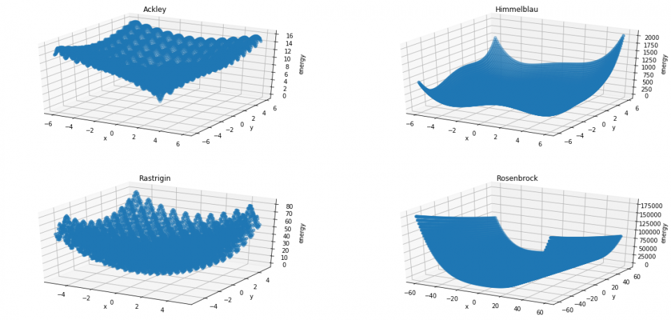
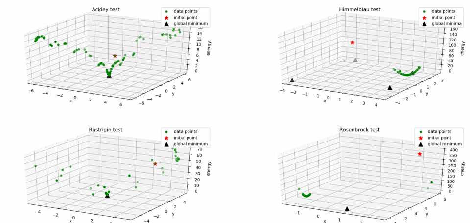
The results are shown in the figure below: we can see the initial point (red star) and the visited states (green dots), while the black triangles are the global minima of the functions. I also reported some useful running information:

Function: Ackley
Stopping criterion: Tolerance
Number of iterations: 1274
Reanniling: False


Function: Himmelblau
Stopping criterion: Tolerance
Number of iterations: 1284
Reanniling: True


Function: Rastrigin
Stopping criterion: Tolerance
Number of iterations: 1315
Reanniling: False


Function: Rosenbrock
Stopping criterion: Tolerance
Number of iterations: 1327
Reanniling: False

The algorithm easily converges in Himmelblau’s test, while it shows some difficulties with Ackley and Rastrigin: the large number of local minima slows down the search. It’s interesting to observe the algorithm behaviour in Rosenbrock test: the test function is very flat and so SA is unable to reach the global minimum before the Energy Tolerance stopping criterion is met.

Bibliography

[1] Holger H. Hoos, Thomas Stützle, Stochastic Local Search, 2005

[2] Henderson, Darrall & Jacobson, Sheldon & Johnson, Alan. (2006). The Theory and Practice of Simulated Annealing. .